Goal
- install python and conda tools on your machine
- install jupyter notebook
- install R and R Studio
- learn to navigate your computer’s file structures from the command line
Introduction
READ THROUGH BEFORE CLICKING/DOING ANYTHING!
Cost = $0.
Anaconda is a platform for data science work. By installing the full Anaconda suite, you get access to a series of tools for working in both the Python and R programming languages, plus excellent visual interfaces that reduce (some of) the pain of programming.
When we do work in Python, we sometimes need to add more lego-pieces to what we’re doing, to accomplish specific tasks. Anaconda comes with very nearly - but not all - of the pieces you might ever need. The thing is, different tasks might require the same pieces, and if you’ve ever fought with a sibling over who gets the good lego piece, well, that’s what can happen inside your machine. Anaconda keeps everything playing nice by allowing us to create environments with copies of the pieces we need, separate from other copies, so that there are no conflicts.
Anaconda also gives us some excellent user interfaces for doing our work - juypter notebooks and R Studio - for instance. But… for our purposes, the full Anaconda installation, with all of its features, is more than what we need. In my experience, students’ computers are littered with lots of software rarely used and rarely uninstalled; so if I ask you to install Anaconda with all of its features, we sometimes run into trouble. You might want it, eventually, but for now, we’re going to use a stripped down version called ‘Miniconda’ which will give us Python and some ‘package managers’.
Python is the basic language, while a package manager lets us retrieve bundles of python code that have been developed for particular tasks, like working with tabular data efficiently. We’ll also use a package manager to install Jupyter Notebooks.
Download Miniconda
- Go to https://docs.conda.io/en/latest/miniconda.html and download the Python 3.8 installer for your computer. Run the installer and accept the defaults.
The first part of this video by former student Chantal Brousseau might be helpful (ignore the second part about ‘environments’ for now):
Anaconda Prompt and Terminal
When I ask you to use the ‘command prompt’ or the ‘terminal’, I am referring to the program that allows you to enter commands directly to your computer through typing.
-
Windows users: I mean “anaconda prompt”. Windows has several different ‘command prompts’ (and also something called ‘powershell’. In these course materials, which have evolved over the years, you’ll see me use a variety of synonyms; understand that I always want you to use the “anaconda prompt”. You can find it in your list of programs/start menu. Again, this is different than the program on your machine called ‘command prompt’. The difference is that the Anaconda prompt knows where your python is installed, while the vanilla command prompt does not.
-
Mac users can use the terminal (which you can find under applications -> other -> terminal).
Going forward, when I want you to enter code at the command prompt or terminal prompt, I will signal this by starting the line with a $, like this:
$ echo "this is what it looks like"
You do not type the $.
- Open a command prompt or terminal now and confirm that miniconda is installed:
$ conda --version
- confirm that python is installed:
$ python --version
if you get an error message, then miniconda did not install correctly or Windows users you might not be in anaconda prompt.
When we type ‘conda’ or ‘python’ or indeed ‘echo’ or anything else at the prompt, we are telling the computer that this is a command. If we want the machine to run a particular python program we’ve written, we would invoke python followed by the program name, eg example.py so that the machine knows to open example.py with python.
Install Jupyter Notebooks
JupyterLab is the latest web-based interactive development environment for notebooks, code, and data. Its flexible interface allows users to configure and arrange workflows in data science, scientific computing, computational journalism, and machine learning. A modular design invites extensions to expand and enrich functionality.
We will use the Jupyter interface with ‘computational notebooks’ from time to time in this class. A computational notebook is a text document where you write your observations and workflow integrated with snippets of code that can be run as you read the document. This allows you to create interactive documents that work with historical data.
- At your computer’s prompt/terminal, install jupyter lab with:
$ pip install notebook
-
Say ‘yes’ to any prompts that might pop up.
-
Test to see that it installed properly:
$ jupyter notebook
A new tab will open in your browser showing the jupyter file explorer interface for the directory where you invoked the jupyter notebook command.
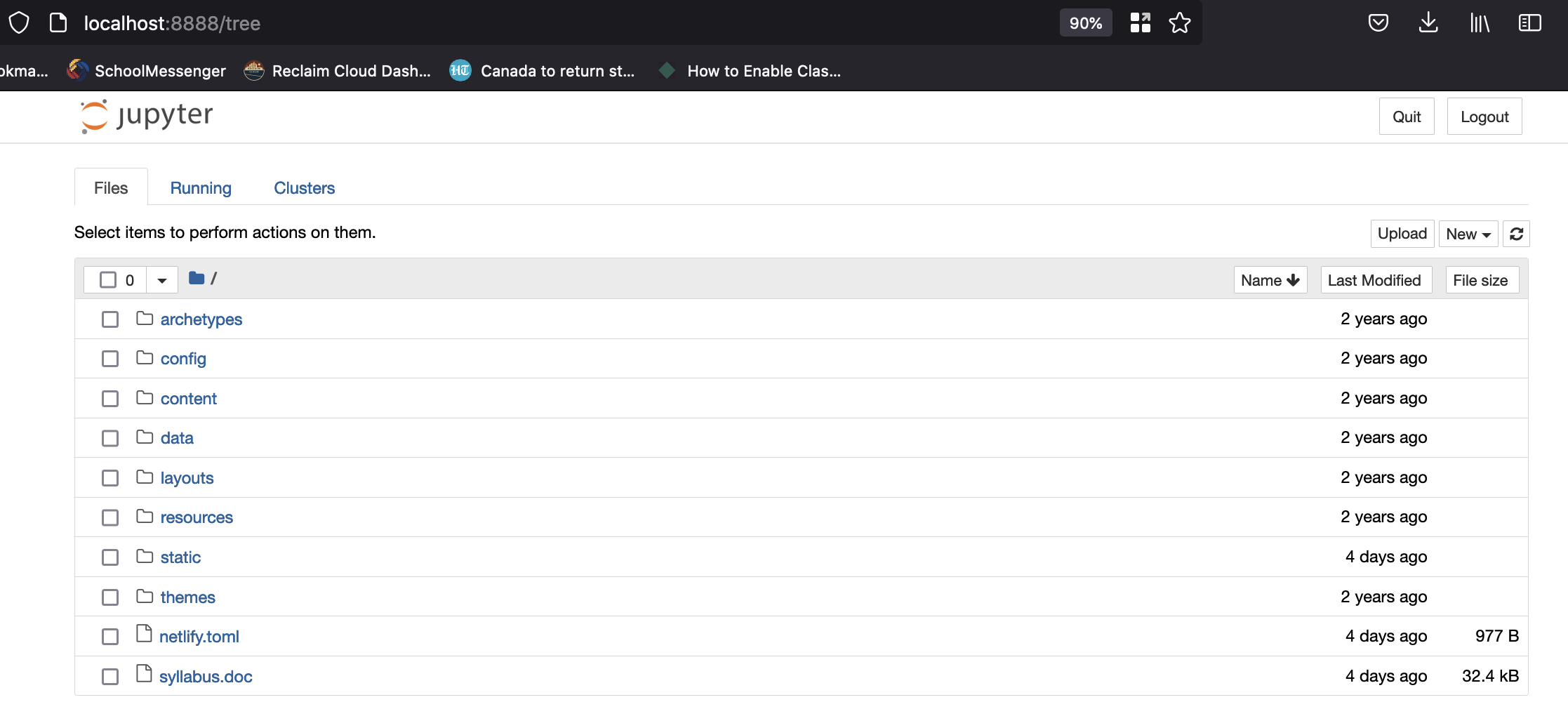
This is what the jupyter file explorer looks like on my machine when I invoke it in the folder where I’m writing all these course materials. Go ahead and click on the ‘new’ dropdown and create a new ‘python notebook’ if you want to play.
Notice the first part of the address in the address bar of my browser: localhost:8888. This is an address not on the web, but on your own personal computer. The Jupyter notebook is running as a ‘web server’ from the directory/folder you make the jupyter notebook command at, and is making jupyter and any of the work you do visible through your web browser through ‘port 8888’. In essence, instead of building a graphical user interface and running as a separate app, Jupyter is borrowing your browser to handle interaction (and to enable you to easily access the wider resources of the web if you need ‘em). We will encounter other software that similarly runs as a ‘web server’.
You can close the tab; in your command prompt or terminal, hit ctrl + c and say ‘yes’ to the ‘shut down notebook server?’ prompt.
Install R and R Studio
R is a language for statistical computing that we will use from time to time. R Studio is an ‘integrated development environment’ or user interface for working with R code, datasets, variables, and plots.
- Mac users download the R programming language here
- Windows users download the R programming language here
You now have a new app on your machine called the ‘R Console’ - you can go ahead and run that, if you want. It will look like this:
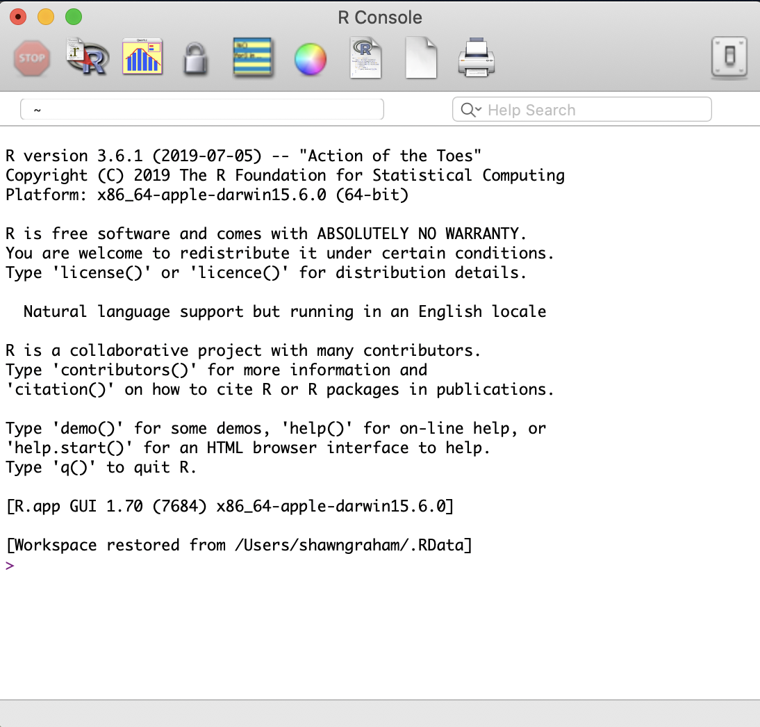
(If you see any text in read giving you some sort of error message in your R console, just copy that text and email me and I’ll walk you through fixing it. This isn’t likely to happen though).
You could use the R console to develop and run R code, but it isn’t… easy. R Studio makes the process less painful.
- Go to the R Studio website and download the installer version of R Studio appropriate for your computer (NOT the ‘tarballs’). Once everything has installed, you can start R Studio up and it should look similarly to this:
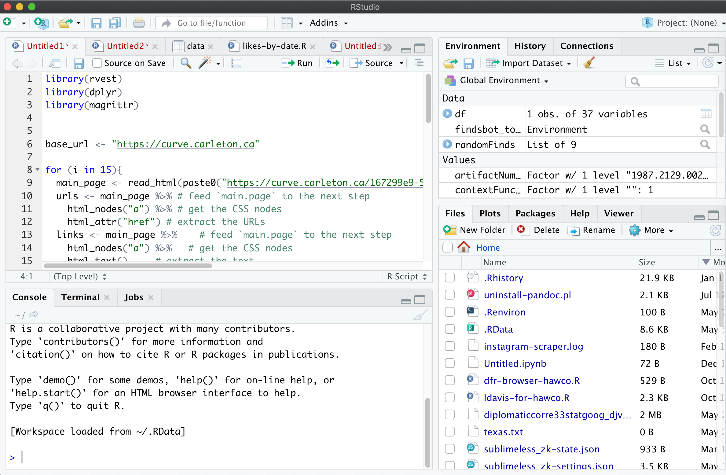
A very busy R Studio interface on my machine, with script (R code) and data files open, a panel showing variables I have created, a file explorer, and the actual code terminal that runs the script files through R. Yours will be a bit more empty than all of this… for now.
Navigating the Command line / terminal
Look at you. You’ve installed a bunch of very cool, very powerful, tools for doing digital history on your computer! The remainder of this tutorial provides some guidance to navigating the structure of how files and folders on your computer are organized. This is very important. When you don’t know or understand how information is organized on your machine, you will run into ‘file not found’ errors that will drive you to distraction. So let’s begin.
When you click on a file in your windows explorer or in mac’s finder, you click through nested folders, right? The path you take through those folders will look something like this: username\example-folder\a-subfolder\file.txt, although finder or explorer by default don’t show you that.
When you open anaconda prompt or the terminal, how do you know where you are at? You print the working directory.
- Try this out:
$ pwd
and that will give you the path to where you are working.
- To see what’s inside the folder, you can try:
$ ls list files, on a Mac or
$ dir directory, on a PC
Files will have an extension (eg, .txt, .doc) while directories won’t. To go into a directory, we change directories.
- Try this (where ‘subfolder’ is one of the folders you saw from running the previous command):
$ cd subfolder
and we can go back up a level:
$ cd ..
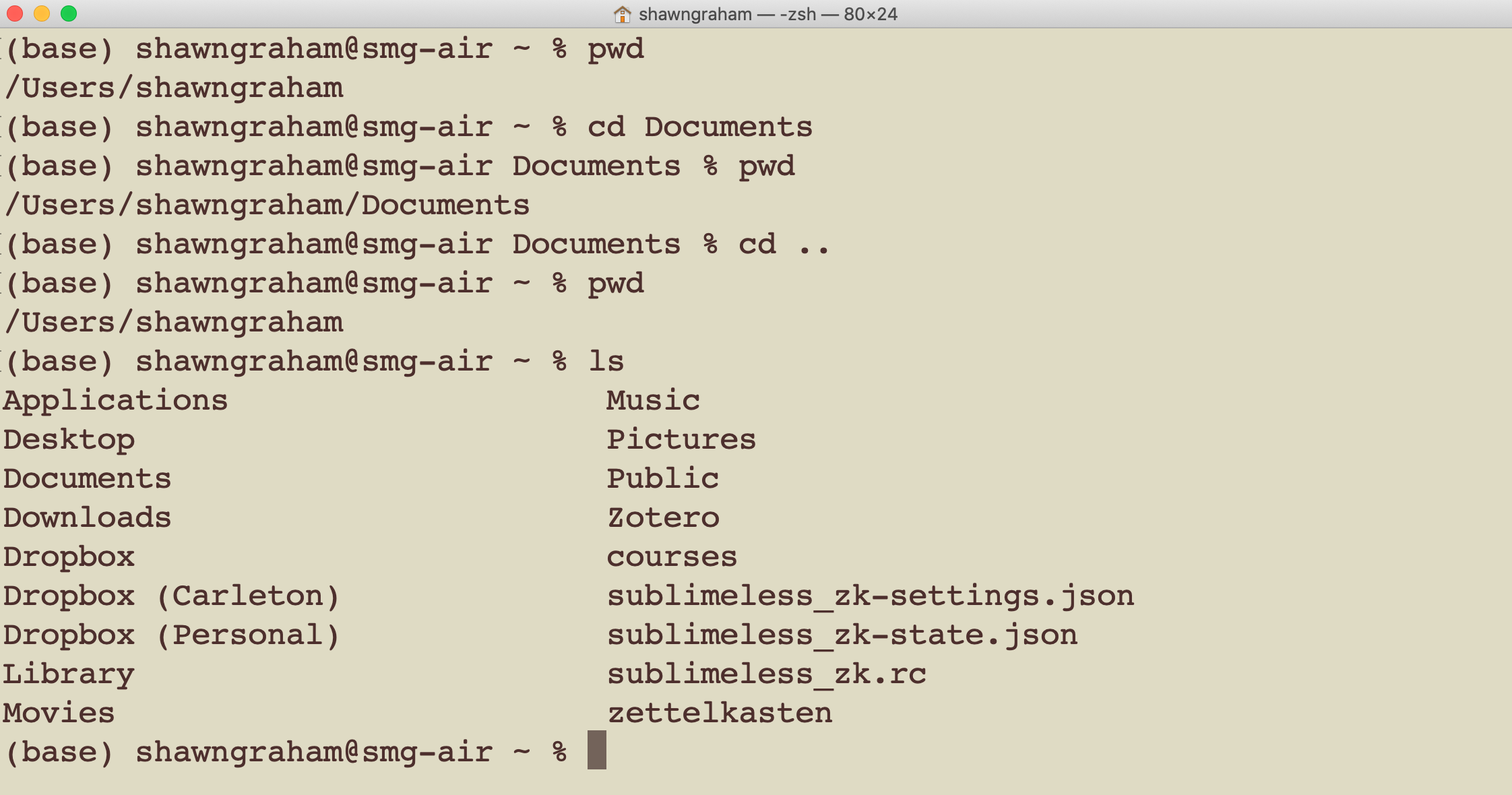
My terminal, demonstrating a bit of moving around. Also some of the contents of my machine.
That wasn’t hard! But there’s more to it, if you care to explore further: